Finite Difference Time Domain Electromagnetics Simulation

this repository uses the FDTD method to model the evolution of some 3d (or 2d) grid-volume of space over time. simulations are seeded with:

• some material at each position in the grid
• a set of stimuli to apply at specific regions in the volume over time
• a set of "measurements" to evaluate and record as the simulation evolves
• an optional state file to allow pausing/resumption of long-run simulations

after this the simulation is advanced in steps up to some user-specified moment in time. measurements are streamed to disk as the simulation runs, so the user can analyze those as the simulation progresses or completes.

Example Usage

simulations are defined by creating binary crate which links against the coremem library. examples are in the crates/applications/ directory. here's an excerpt from the wavefront example:

// use a general-purpose material, capable of representing vacuum, conductors, and magnetic materials.
type Mat = mat::GenericMaterial<f32>;

// simulate a volume of 401x401x1 discrete grid cells.
let (width, height, depth) = (401, 401, 1);
let size = Index::new(width, height, depth);
// each cell represents 1um x 1um x 1um volume.
let feature_size = 1e-6;

// create the simulation "driver".
// the first parameter is the float type to use: f32 for unchecked math, coremem::real::R32
// to guard against NaN/Inf (useful for debugging).
// to run this on the gpu instead of the gpu, replace `CpuBackend` with `WgpuBackend`.
let mut driver = Driver::new(SpirvSim::<f32, Mat, spirv::CpuBackend>::new(size, feature_size));

// create a conductor on the left side.
let conductor = Cube::new(
    Index::new(0, 0, 0).to_meters(feature_size),
    Index::new(width/10, height, 1).to_meters(feature_size),
);
driver.fill_region(&conductor, mat::IsomorphicConductor::new(200f32));

// create a vertical strip in the center of the simulation which emits a wave.
let center_region = Cube::new(
    Index::new(200, height/4, 0).to_meters(feature_size),
    Index::new(201, height*3/4, 1).to_meters(feature_size),
);

// emit a constant E/H delta over this region for 100 femtoseconds
let stim = ModulatedVectorField::new(
    RegionGated::new(center_region, Fields::new_eh(
        Vec3::new(2e19, 0.0, 0.0),
        Vec3::new(0.0, 0.0, 2e19/376.730),
    )),
    Pulse::new(0.0, 100e-15),
);
driver.add_stimulus(stim);

// finally, run the simulation through t=100ps
driver.step_until(Seconds(100e-12));

you can run the full example with:

$ cargo run --release --bin wavefront

graphical simulation output is displayed directly to the terminal, and also rendered (in higher resolution) to a video file in out/applications/wavefront/.

this example runs on the CPU. the moment you do anything more complex than this, you'll want to leverage the GPU, which can easily be 30-100x faster:

GPU Acceleration

we use rust-gpu for gpu acceleration. presently, this requires specific versions of rust-nightly to work. the feature is toggled at runtime, but compiled unconditionally. set up the toolchain according to rust-toolchain.toml:

$ rustup default nightly-2022-08-29
$ rustup component add rust-src rustc-dev llvm-tools-preview

now you can swap out the CpuDriver with a SpirvDriver and you're set:

-    let mut driver = Driver::new(SpirvSim::<f32, Mat, spirv::CpuBackend>::new(size, feature_size));
+    let mut driver = Driver::new(SpirvSim::<f32, Mat, spirv::WgpuBackend>::new(size, feature_size));

re-run it as before and you should see the same results:

$ cargo run --release --example wavefront

see the "Processing Loop" section below to understand what GPU acceleration entails.

Advanced Usage: Viewers, Measurements

the sr_latch example explores a more interesting feature set. first, it "measures" a bunch of parameters over different regions of the simulation (peak inside crates/coremem/src/meas.rs to see how these each work):

// measure a bunch of items of interest throughout the whole simulation duration:
driver.add_measurement(meas::CurrentLoop::new("coupling", coupling_region.clone()));
driver.add_measurement(meas::Current::new("coupling", coupling_region.clone()));
driver.add_measurement(meas::CurrentLoop::new("sense", sense_region.clone()));
driver.add_measurement(meas::Current::new("sense", sense_region.clone()));
driver.add_measurement(meas::MagneticLoop::new("mem1", ferro1_region.clone()));
driver.add_measurement(meas::Magnetization::new("mem1", ferro1_region.clone()));
driver.add_measurement(meas::MagneticFlux::new("mem1", ferro1_region.clone()));
driver.add_measurement(meas::MagneticLoop::new("mem2", ferro2_region.clone()));
driver.add_measurement(meas::CurrentLoop::new("set", set_region.clone()));
driver.add_measurement(meas::Current::new("set", set_region.clone()));
driver.add_measurement(meas::Power::new("set", set_region.clone()));
driver.add_measurement(meas::CurrentLoop::new("reset", reset_region.clone()));

during the simulation, it dumps these measurements into a CSV:

// render a couple CSV files: one very detailed and the other more sparsely detailed
driver.add_csv_renderer(&*format!("{}meas.csv", prefix), 200, None);
driver.add_csv_renderer(&*format!("{}meas-sparse.csv", prefix), 1600, None);

furthermore, it serializes point-in-time snapshots of the simulation while it's running, allowing you to dig further into the simulation in an interactive way (versus the raw video renderer used in the wavefront example):

// serialize frames for later viewing with `cargo run --release --bin viewer`
driver.add_serializer_renderer(&*format!("{}frame-", prefix), 36000, None);

run this, after having setup the GPU pre-requisites:

$ cargo run --release --example sr_latch

and then investigate the results with

$ cargo run --release --bin viewer ./out/applications/sr_latch

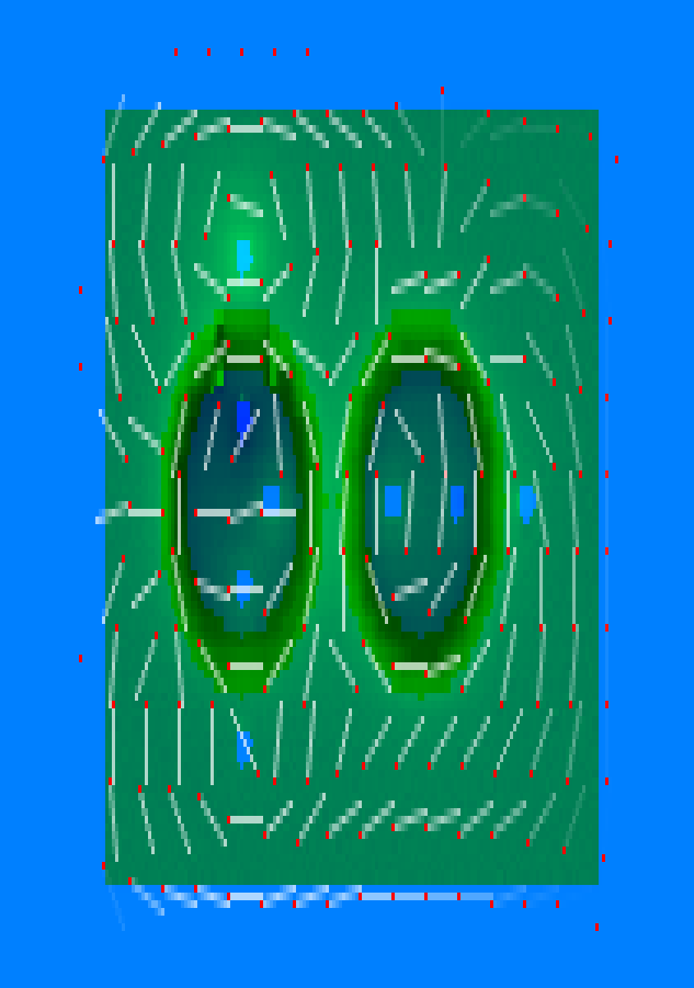
the viewer shows us a single xy cross-section of the simulation at a moment in time. it uses red-tipped arrows to show the x-y components of the B field at every point, and the Z component of the E field is illustrated with color (bright green for positive polarization and dark blue for negative). the light blue splotches depict the conductors (in the center, the wire coupling loops; on the edge, our energy-dissipating boundary).

what we see here is that both ferrites (the two large circles in the above image) have a clockwise polarized B field. this is in the middle of a transition, so the E fields look a bit chaotic. advance to t=46 ns: the "reset" pulse was applied at t=24ns and had 22ns to settle:

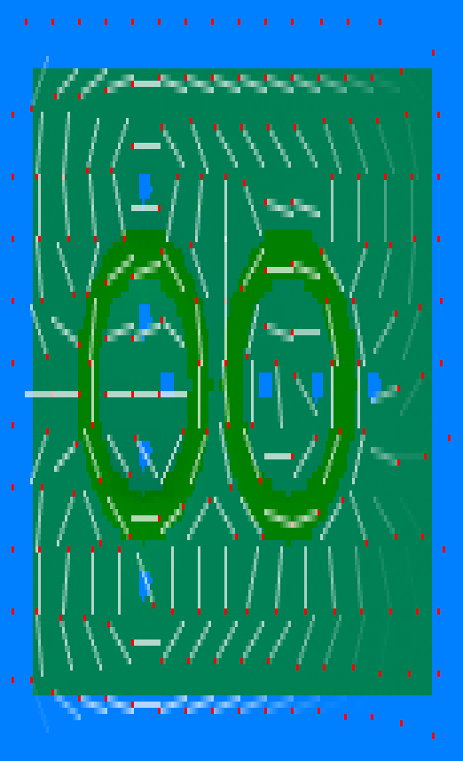
we can see the "reset" pulse has polarized both ferrites in the counter-clockwise orientation this time. the E field is less pronounced because we gave the system 22ns instead of 3ns to settle this time.

the graphical viewer is helpful for debugging geometries, but the CSV measurements are useful for viewing numeric system performance. peak inside "out/applications/sr-latch/meas.csv" to see a bunch of measurements over time. you can use a tool like Excel or visidata to plot the interesting ones.

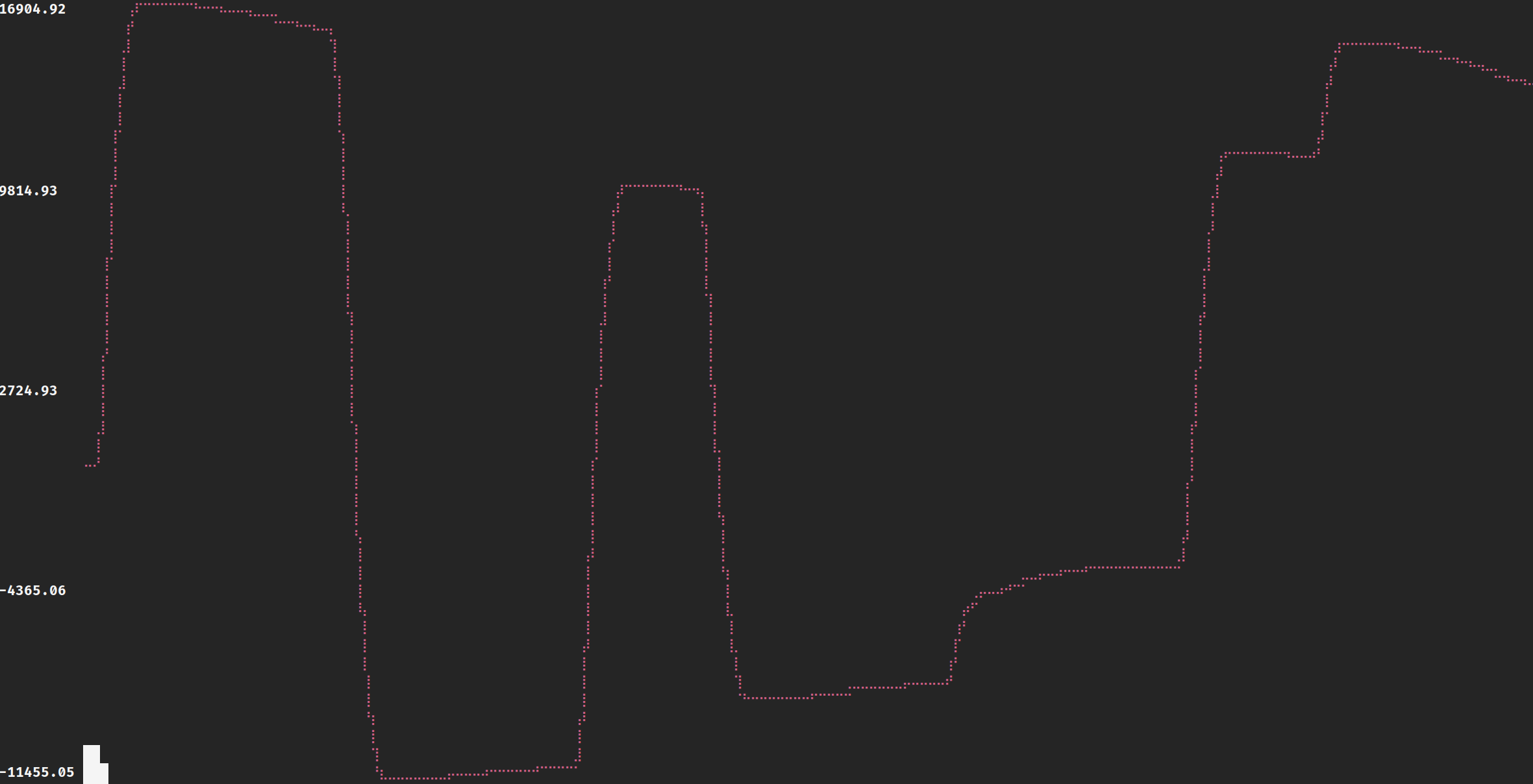
here's a plot of M(mem2) over time from the SR latch simulation. we're measuring, over the torus volume corresponding to the ferrite on the right in the images above, the (average) M component normal to each given cross section of the torus. the notable bumps correspond to these pulses: "set", "reset", "set", "reset", "set+reset applied simultaneously", "set", "set".

Processing Loop (and how GPU acceleration works)

the processing loop for a simulation is roughly as follows (crates/coremem/src/driver.rs:step_until drives this loop):

1. evaluate all stimuli at the present moment in time; these produce an "externally applied" E and H field across the entire volume.
2. apply the FDTD update equations to "step" the E field, and then "step" the H field. these equations take the external stimulus from step 1 into account.
3. evaluate all the measurement functions over the current state; write these to disk.
4. serialize the current state to disk so that we can resume from this point later if we choose.

within each step above, the logic is multi-threaded and the rendeveous points lie at the step boundaries.

it turns out that the Courant rules force us to evaluate FDTD updates (step 2) on a far smaller time scale than the other steps are sensitive to. so to tune for performance, we apply some optimizations:

• stimuli (step 1) are evaluated only once every N frames. we still apply them on each frame individually. the waveform resembles that of a Sample & Hold circuit.
• measurement functions (step 3) are triggered only once every M frames.
• the state is serialized (step 4) only once every Z frames.

N, M, and Z are all tunable by the application.

as a result, step 2 is actually able to apply the FDTD update functions not just once but up to min(N, M, Z) times. although steps 1 and 3 vary heavily based on the user configuration of the simulation, step 2 can be defined pretty narrowly in code (no user-callbacks/dynamic function calls/etc). this lets us offload the processing of step 2 to a dedicated GPU. by tuning N/M/Z, step 2 becomes the dominant cost in our simulations and GPU offloading can easily boost performance by more than an order of magnitude on even a mid-range consumer GPU.

Features

this library takes effort to separate the following from the core/math-heavy "simulation" logic:

• Stimuli
• Measurements
• Render targets (video, CSV, etc)
• Materials (conductors, non-linear ferromagnets)
• Float implementation

the simulation only interacts with these things through a trait interface, such that they're each swappable.

common stimuli type live in crates/coremem/src/stim/. common measurements live in crates/coremem/src/meas.rs. common render targets live in crates/coremem/src/render.rs. these change infrequently enough that crates/coremem/src/driver.rs has some specialized helpers for each render backend. common materials are spread throughout crates/cross/src/mat/. different float implementations live in crates/cross/src/real.rs. if you're getting NaNs, you can run the entire simulation on a checked R64 (CPU-only) or R32 (any backend) type in order to pinpoint the moment those are introduced.

Materials

each cell is modeled as having a vector E, H and M field, as well as a Material type defined by the application.

the Material trait has the following methods (both are optional):

pub trait Material<R: Real>: Sized {
    fn conductivity(&self) -> Vec3<R>;
    /// returns the new M vector for this material. called during each `step_h`.
    fn move_b_vec(&self, m: Vec3<R>, target_b: Vec3<R>) -> Vec3<R>;
}

to add a new material:

• for CpuBackend simulations: just implement this trait on your own type and instantiate a SpirvSim specialized over that material instead of GenericMaterial.
• for WgpuBackend simulations: do the above and add a spirv entry-point specialized to your material. scroll to the bottom of crates/spirv_backend/src/lib.rs and follow the examples.

as can be seen, the Material trait is fairly restrictive. its methods are immutable, and it doesn't even have access to the entire cell state (only the cell's M value, during move_b_vec). i'd be receptive to a PR or request that exposes more cell state or mutability: this is just an artifact of me tailoring this specifically to the class of materials i intended to use it for.

What's in the Box

this library ships with the following materials:

• conductors (Isomorphic or Anisomorphic).
• a handful of ferromagnet implementations:
  • MHPgram specifies the M(H) function as a parallelogram.
  • MBPgram specifies the M(B) function as a parallelogram.

measurements include (crates/coremem/src/meas.rs):

• E, B or H field (mean vector over some region)
• energy, power (net over some region)
• current (mean vector over some region)
• mean current magnitude along a closed loop (toroidal loops only)
• mean magnetic polarization magnitude along a closed loop (toroidal loops only)

output targets include (crates/coremem/src/render.rs):

• ColorTermRenderer: renders 2d-slices in real-time to the terminal.
• Y4MRenderer: outputs 2d-slices to an uncompressed y4m video file.
• SerializerRenderer: dumps the full 3d simulation state to disk. parseable after the fact with crates/post/src/bin/viewer.rs.
• CsvRenderer: dumps the output of all measurements into a csv file.

historically there was also a plotly renderer, but that effort was redirected into developing the viewer tool better.

Performance

with my Radeon RX 5700XT, the sr_latch example takes 125 minutes to complete 150ns of simulation time (3896500 simulation steps). that's on a grid of size 163x126x80 where the cell dimension is 20um.

in a FDTD simulation, as we shrink the cell size the time step has to shrink too (it's an inverse affine relationship). so the scale-invariant performance metric is "grid cell steps per second" ((163*126*80)*3896500 / (125*60)): we get 850M.

this is the "default" optimized version. you could introduce a new material to the simulation, and performance would remain constant. as you finalize your simulation, you can specialize it a bit and compile the GPU code to optimize for your specific material. this can squeeze another factor-of-2 gain: view buffer_proto5 to see how that's done.

contrast that to the CPU-only implementation which achieves 24.6M grid cell steps per second on my 12-core Ryzen 3900X: that's about a 34x gain.

Support

the author can be reached on Matrix <@colin:uninsane.org>, email colin@uninsane.org or Activity Pub <@colin@fed.uninsane.org>. i poured a lot of time into making this: i'm happy to spend the marginal extra time to help curious people make use of what i've made, so don't hesitate to reach out.

Additional Resources

this whole library is really just an implementation of the Finite Difference Time Domain method with abstractions atop that to make it useful.

John B. Schneider has an extremely detailed beginner's guide for implementing FDTD from start to finish:

• John B. Schneider: Understanding the Finite-Difference Time-Domain Method

Gregory Werner and John Cary provide a more rigorous approach and include error measurements which are useful for validation:

• Gregory Werner, John Cary: A stable FDTD algorithm for non-diagonal, anisotropic dielectrics (2007)

MEEP is another open-source FDTD project. it has quality docs which i used as a starting point in my research.

David Bennion and Hewitt Crane documented their approach for transforming Diode-Transistor Logic circuits into magnetic core circuits:

• David Bennion, Hewitt Crane: All-Magnetic Circuit Techniques (1964)

although i decided not to use PML, i found Steven Johnson's (of FFTW fame) notes to be the best explainer of PML:

• Steven Johnson: Notes on Perfectly Matched Layers (PMLs)

a huge thanks to everyone above for sharing the fruits of their studies. though my work here is of a lesser caliber, i hope that someone, likewise, may someday find it of use.